How Hidden Volatility Feedback Loops Determine Your P&L: The Multivariate Quadratic Hawkes Revolution

---

TL;DR: Volatility isn’t just path-dependent — it responds quadratically to past trends across multiple assets. Recent empirical work on Multivariate Quadratic Hawkes Processes (Aubrun et al., 2023, 2025) reveals that E-mini futures trends drive idiosyncratic stock volatility universally, past covariance between assets feeds forward into future volatility, and cross-leverage effects create systematic opportunities that local volatility models completely miss. Understanding these mechanisms explains why certain volatility trades work and others fail catastrophically.

The Multi-Billion Dollar Problem With Local Volatility

Every volatility trader knows the uncomfortable truth: local volatility models, which assume volatility depends only on the current asset price and not the path taken to reach it, are fundamentally flawed. Yet billions in derivatives continue to be priced using these models.

The flaw isn’t subtle. When you sell volatility using a local vol framework, you’re implicitly assuming the market has no memory — that a stock at $100 after trending up 10% looks identical to the same stock at $100 after whipsawing violently. Market data reveals this assumption is catastrophically wrong: volatility depends fundamentally on the path of recent price changes (Guyon, 2022; Chicheportiche & Bouchaud, 2014).

This path dependence creates systematic profit opportunities for those who understand it — and systematic losses for those who don’t.

Two Types of Path Dependence You Must Know

The Leverage Effect: Directional Memory

The leverage effect describes how negative returns increase future volatility while positive returns dampen it. Bouchaud, Matacz & Potters (2001) document that for individual stocks, this correlation is moderate and decays over 50 days, while for stock indices it is much stronger but decays faster. For the S&P 500, this effect is pronounced and well-established (Black, 1976).

P&L Implication: Selling volatility after market declines systematically underprices risk. The volatility you sold at 20 VIX will likely realize at 25+ if the selloff continues — even if the spot price stabilizes. This is not a statistical fluke; it’s a structural feature of how volatility forms.

The Zumbach Effect: Trend-Magnitude Feedback

The Zumbach effect captures the empirical property that past squared returns forecast future volatilities better than past volatilities forecast future squared returns (El Euch & Rosenbaum, 2019; Zumbach, 2009). In plain English: large trends — regardless of direction — increase future volatility.

When unexplained local trends emerge, liquidity providers become wary that informed traders know something they don’t, leading to wider spreads and increased volatility (Bouchaud, 2022). For small trends, you get the leverage effect (down = higher vol). For large trends of either sign, you get the Zumbach effect (big move = higher vol).

Standard linear Hawkes processes fail to reproduce the observed quadratic path-dependency and the Zumbach effect when calibrated to real data; adding quadratic terms resolves these mismatches (Blanc, Donier & Bouchaud, 2017). This is where Quadratic Hawkes Processes become essential.

The Mathematics of Money: Quadratic Hawkes Processes

The Core Mechanism

Quadratic Hawkes (QHawkes) models generalize standard Hawkes processes by allowing feedback effects that are both linear and quadratic in past returns (Blanc et al., 2017). The jump intensity becomes:

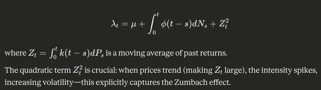
Why This Model Matters for P&L

QHawkes models exhibit two properties critical for volatility modeling (Blanc et al., 2017):

1. Time-reversal asymmetry matching financial markets’ preferred directional evolution

2. Generation of multiplicative, fat-tailed volatility processes

Non-parametric fits on NYSE stock data show the off-diagonal component of the quadratic kernel has structure that standard linear Hawkes models fail to reproduce (Blanc et al., 2017).

The Edge: If your volatility model assumes time-reversal symmetry — like CIR-Heston or classical stochastic vol models, which obey time-reversal symmetry by construction (El Euch & Rosenbaum, 2019) — you’re systematically mispricing options because these models cannot account for the observed time-reversal asymmetry of financial time series.

The Multivariate Revolution: Cross-Market Feedback Loops

Single-asset QHawkes is powerful. The multivariate extension (MQHawkes) — motivated by strong empirical evidence of endogenous co-jumps where multiple assets jump simultaneously — reveals an entirely new layer of market structure (Aubrun, Benzaquen & Bouchaud, 2023).

Three New Effects That Drive P&L

1. Cross-Zumbach Effects: Index Trends Drive Individual Stock Vol

Aubrun et al. (2025) provide the first clear identification of cross-Zumbach effects: the effect of recent trends of E-mini futures contracts on the volatility of other futures contracts is especially strong. This isn’t correlation — it’s a causal feedback mechanism within the MQHawkes framework.

The Trade: When E-mini futures trend heavily (regardless of direction), implied volatility on correlated assets systematically underprices the coming realized volatility spike. You want to be long gamma across the complex.

2. Covariance-to-Volatility Feedback: A New Risk Factor

A new feedback type couples past realized covariance between two assets and future volatility of these same assets, with E-mini/T-bond as a prime example (Aubrun et al., 2025).

When E-mini and T-bonds move together unusually (high realized covariance), future volatility in both assets rises. The Yule-Walker equations relating covariances and feedback kernels are essential to calibrate the MQHawkes process on empirical data (Aubrun et al., 2023).

The Trade: Monitor realized correlation between E-mini and T-bonds in real-time. When it spikes above historical norms, implied vols on both are about to underprice realized vol. Standard dispersion trades miss this entirely.

3. Universal Cross-Leverage: Index Moves Drive Idiosyncratic Vol

Here’s the crown jewel finding.

When the index goes down, the idiosyncratic part of individual stock volatility also goes up — and this cross-leverage effect between E-mini and residual stock volatility is remarkably universal across stocks (Aubrun et al., 2025).

The empirical kernel (Figure 9 in Aubrun et al., 2025) starts around -0.1 at short lags and asymptotes toward zero over approximately 20 time units. The grey uncertainty band is barely visible — meaning this effect is consistent across hundreds of stocks.

The Critical Implication: When you’re hedging single-stock volatility with index options, you’re not just hedging systematic risk — you’re hedging a structural feedback mechanism where index returns directly amplify idiosyncratic volatility.

Why Standard Models Lose Money Here

Traditional approaches treat:

• Systematic and idiosyncratic volatility as independent

• Cross-asset effects as pure correlation

• Volatility as depending only on its own past dynamics

All of these assumptions are empirically false when you examine the non-parametric calibration of MQHawkes on high-frequency data (Aubrun et al., 2025).

The Practical Edge: Calibration and Implementation

Non-Parametric Calibration

Assuming quadratic kernels decompose as the sum of a time-diagonal component and a rank-one trend contribution allows investigation of endogeneity ratios and resulting stationarity conditions (Aubrun et al., 2023).

The time-diagonal part captures standard Hawkes feedback (activity begets activity). The rank-one trend component captures path dependency — specifically how past price trends influence future activity.

Stationarity Constraints

The volatility distribution exhibits power-law behavior with an exponent that can be exactly computed in limiting cases (Aubrun et al., 2023). For the process to remain stationary, the endogeneity ratio must stay below unity.

Risk Management Implication: When markets approach critical regimes (endogeneity ratio → 1), small perturbations can trigger large volatility cascades. Empirical calibrations report average endogeneity around 0.96 in some regimes (Aubrun et al., 2025) — dangerously close to the critical threshold. This explains flash crashes and why “tail risk” events cluster.

Real-Time Application

Real-time Hawkes volatility measures allow traders to observe market volatility of each stock continuously, useful for managing intraday price risk (Lee & Seo, 2024).

During the 2015 Chinese stock market crash, adding Hawkes indicators to HAR models improved both in-sample and out-of-sample volatility forecasts for 300 major stocks (Fan et al., 2023).

When volatility spikes, your model needs to capture why. Is it:

• Past volatility feeding forward (GARCH-type)?

• Recent trends creating uncertainty (Zumbach)?

• Cross-market contagion (multivariate Hawkes)?

• All three?

MQHawkes gives you the decomposition.

Connecting to Rough Volatility

Scaling limits of Quadratic Hawkes processes with power-law kernels yield super-rough-Heston models that preserve time-reversal asymmetry (Dandapani, Jusselin & Rosenbaum, 2021). While the Zumbach effect is negligible in classical Heston, it’s consistent with empirical estimates under rough Heston (El Euch & Rosenbaum, 2019).

This connects microstructure (tick-by-tick QHawkes) to derivatives pricing (rough vol models). The path from microscopic to macroscopic behavior is no longer a mystery — it’s a mathematical derivation.

How Money Is Made (and Lost)

What Works

1. Trend-Conditional Vol Trading

• Buy volatility when trends are large (either direction) and implied vol is low

• Sell volatility only after extended low-trend regimes

• Never ignore the quadratic term

2. Cross-Market Vol Arbitrage

• When E-mini trends hard, buy vol on correlated single names

• When E-mini/T-bond covariance spikes, prepare for vol expansion in both

• Use MQHawkes feedback kernels to size positions

3. Dispersion Trades with Cross-Leverage

• Traditional index vs. single-stock dispersion assumes independence

• Cross-leverage effects create systematic bias in dispersion pricing

• Adjust strikes and position sizing for universal cross-leverage

4. Real-Time Risk Management

• Hawkes-based market-making strategies trained with adversarial reinforcement learning adapt to high-volatility regimes while maintaining stable bid-ask quoting (Wang et al., 2025)

• Monitor endogeneity ratios approaching unity — signal for risk reduction

• Use intensity process to forecast short-term clustering

What Fails

1. Local Vol Deltas

• Your hedge ratios are wrong if you ignore path dependence

• After a 5% down move, spot may recover but vol stays elevated

• P&L bleeds from unhedged path-dependent risk

2. Ignoring Cross-Asset Feedback

• Hedging single stocks with index ignoring cross-leverage = unhedged exposure

• Assuming covariance doesn’t feed forward to volatility = structural bias

• Missing cross-Zumbach = systematically wrong on correlation trades

3. Time-Reversal Symmetric Models

• CIR-Heston and classical stochastic vol models obey time-reversal symmetry by construction, failing to capture observed time-reversal asymmetry (El Euch & Rosenbaum, 2019)

• Pricing long-dated options with symmetric models = structural mispricing

• Vega exposure in the wrong direction during regime changes

The Bigger Picture: Why This Matters Now

Interconnectedness between crude oil, stock, and forex markets is shaped by distributional moments, with realized volatility spillovers significantly stronger than higher-order moments (Wang et al., 2025). Spillover dynamics exhibit time-varying behavior highly sensitive to crises including COVID-19, Russia-Ukraine conflict, and Middle East tensions.

We’re in an era of:

• Increased cross-market correlation

• Faster information propagation

• Higher frequency trading

• Greater endogeneity (more feedback loops)

Standard linear Hawkes processes, while capturing some feedback, fail to reproduce the observed quadratic path-dependency when calibrated to real data (Blanc et al., 2017). You need the quadratic extension to capture reality.

Empirical Validation: The Universal Cross-Leverage Kernel

Return to Figure 9 in Aubrun et al. (2025). The cross-leverage kernel between E-mini and residual stock volatility is surprisingly universal — the dispersion across stocks (grey region) is barely visible.

This universality is profound. It means:

1. The effect is structural, not statistical noise

2. It applies broadly across market cap, sector, beta

3. You can build systematic strategies around it

4. Ignoring it creates consistent, measurable alpha leakage

Conclusion: The New Framework for Volatility Trading

Multivariate Quadratic Hawkes Processes aren’t just an academic curiosity — they’re a fundamental reframing of how volatility works:

• Volatility is path-dependent: Past trends matter as much as current price

• The quadratic term is critical: Large moves increase vol regardless of direction

• Cross-market effects are causal: E-mini trends drive single-stock idiosyncratic vol

• Covariance feeds forward: Past correlation between assets predicts future volatility

• The effects are universal: Cross-leverage holds across hundreds of stocks

As in the univariate case, the volatility distribution tail exhibits power-law behavior with a unique exponent that can be exactly computed (Aubrun et al., 2023). This isn’t stochastic — it’s deterministic structure in the market.

The Bottom Line: If your volatility models assume time-reversal symmetry, ignore path dependence, or treat assets independently, you’re systematically mispricing risk. The market’s feedback structure is quadratic, multivariate, and path-dependent. Trade accordingly.

---

References & Further Reading

Core Papers:

• Blanc, P., Donier, J., & Bouchaud, J.P. (2017). “Quadratic Hawkes Processes for Financial Prices.” Quantitative Finance, 17(2), 171–188. arXiv:1509.07710

• Aubrun, C., Benzaquen, M., & Bouchaud, J.P. (2023). “Multivariate Quadratic Hawkes Processes — Part I: Theoretical Analysis.” Quantitative Finance, 23(5), 741–758.

• Aubrun, C., Hey, N., & Benzaquen, M. (2025). “Multivariate Quadratic Hawkes Processes — Part II: Non-Parametric Empirical Calibration.” arXiv:2509.21244.

On the Zumbach Effect:

• El Euch, O., & Rosenbaum, M. (2019). “The Zumbach Effect Under Rough Heston.” Quantitative Finance, 20(2), 235–247. arXiv:1809.02098

• Zumbach, G. (2009). “Time Reversal Invariance in Finance.” Quantitative Finance, 9(5), 505–515.

On Leverage Effects:

• Bouchaud, J.P., Matacz, A., & Potters, M. (2001). “Leverage Effect in Financial Markets: The Retarded Volatility Model.” Physical Review Letters, 87, 228701.

• Black, F. (1976). “Studies of Stock Price Volatility Changes.” Proceedings of the American Statistical Association, Business and Economic Statistics Section, 177–181.

On Path-Dependent Volatility:

• Guyon, J. (2022). “Volatility Is (Mostly) Path-Dependent.” ResearchGate.

• Chicheportiche, R., & Bouchaud, J.P. (2014). “The Fine-Structure of Volatility Feedback I: Multi-Scale Self-Reflexivity.” Physica A, 410, 174–195.

Practical Applications:

• Bacry, E., Mastromatteo, I., & Muzy, J.F. (2015). “Hawkes Processes in Finance.” Market Microstructure and Liquidity, 1(1), 1550005. arXiv:1502.04592

• Lee, K., & Seo, B.K. (2024). “Application of Hawkes Volatility in the Observation of Filtered High-Frequency Price Process.” Applied Stochastic Models in Business and Industry.

• Fan, Y., et al. (2023). “Forecasting Stock Volatility During the Stock Market Crash Period: The Role of Hawkes Process.” Finance Research Letters, 53, 103568.

Scaling Limits:

• Dandapani, A., Jusselin, P., & Rosenbaum, M. (2021). “From Quadratic Hawkes Processes to Super-Heston Rough Volatility Models with Zumbach Effect.” Stochastic Processes and their Applications.

Cross-Market Studies:

• Wang, J., et al. (2025). “Crude Oil, Forex, and Stock Markets: Unveiling the Higher-Order Moment and Cross-Moment Risk Spillovers in Times of Turmoil.” Humanities and Social Sciences Communications.

• Wang, Z., et al. (2025). “ARL-Based Multi-Action Market Making with Hawkes Processes and Variable Volatility.” Proceedings of the 5th ACM International Conference on AI in Finance.

Additional Resources:

• Bouchaud, J.P. (2022). “Volatility and Time Reversal Asymmetry.” Substack

---

About This Series

This article is part of a series deep-diving into quantitative finance concepts with one question: How did this trade make (or lose) money?

Each piece focuses on: ✅ The specific market mechanism at work
✅ How positions are structured and risk-managed
✅ Where P&L comes from (or where it leaks)
✅ Actionable principles for traders and researchers

Follow for more deep dives on real trades, quant strategies, and the mechanics behind hedge fund P&L.

Have thoughts on MQHawkes applications or want to discuss implementation details? Let’s connect in the comments or via DM.

---

Disclaimer: This article is for educational purposes only and does not constitute investment advice. Derivatives trading involves substantial risk of loss.